Magnetostatics
A collection of analytical and semi-analytical calculation tools to evaluate magnetic field from arbitrary coils.
2-D current sources
The following relations are for circular current sources about the \(z\)-axis.
Green’s functions
The Green’s functions for poloidal magnetic flux, radial magnetic field, and vertical magnetic field at a point \((x, z)\) due to a unit current source at point \((x_c, z_c)\):
import numpy as np

from bluemira.magnetostatics.greens import greens_Bx, greens_Bz, greens_psi

coil_x, coil_z = 4, 5
x = np.linspace(0.1, 10, 100)
z = np.linspace(0, 10, 100)
xx, zz = np.meshgrid(x, z)

psi = greens_psi(coil_x, coil_z, xx, zz)
Bx = greens_Bx(coil_x, coil_z, xx, zz)
Bz = greens_Bz(coil_x, coil_z, xx, zz)
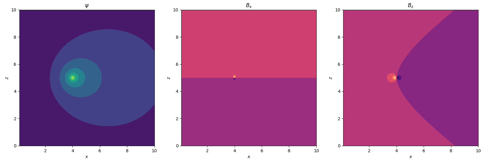
To obtain the actual \(\psi\), \(B_x\), and \(B_z\) in V.s / rad and T, simply multiply the Green’s functions by the current at the source point in Ampères.
Note
The above Green’s functions are effectively for an infinitely thin filament and diverge logarithmically as the evaluation point approaches the source point.
Warning
The above Green’s functions should only be used for \(x\) > 0. Errors and garbage are to be expected for \(x\) <= 0.
Semi-analytical functions
For a circular coil of rectangular cross-section, a semi-analytic reduction of the 3-D Biot-Savart law is used, as developed by [Zhang_2012]. Numerical integration is used in one dimension, and some singularities in the equations are resolved numerically and analytically.
import numpy as np

from bluemira.magnetostatics.semianalytic_2d import (
    semianalytic_Bx,
    semianalytic_Bz,
    semianalytic_psi,
)

coil_x, coil_z = 4, 5
coil_dx, coil_dz = 1, 2
x = np.linspace(0.1, 10, 100)
z = np.linspace(0, 10, 100)
xx, zz = np.meshgrid(x, z)

psi = semianalytic_psi(coil_x, coil_z, xx, zz, coil_dx, coil_dz)
Bx = semianalytic_Bx(coil_x, coil_z, xx, zz, coil_dx, coil_dz)
Bz = semianalytic_Bz(coil_x, coil_z, xx, zz, coil_dx, coil_dz)
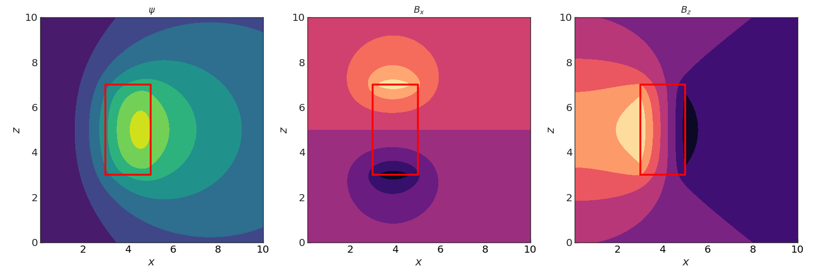
Hint
The above semi-analytical functions are best used for points inside or near the current source. If you favour speed over accuracy, for points further away from the current source, you are better off using some quadratures of Green’s functions.
3-D current sources
Several options are available for calculating magnetic fields due to three-dimensional current sources.
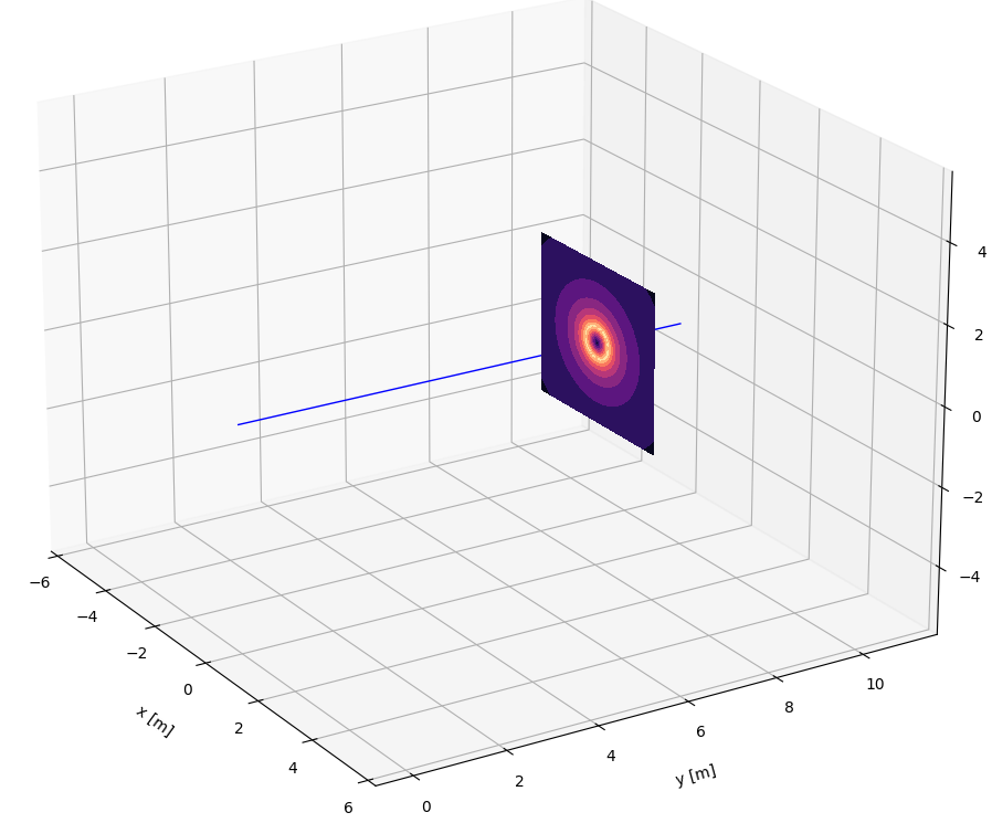
Biot-Savart
The Biot-Savart equation
can be solved assuming the current sources are thin wires, as is done in the
BiotSavartFilament object.
A radius argument can be specified, which makes use of a square decay law for values
inside the filament radius. The field from a filament thus reaches a maximum at the
surface of the filament.
import matplotlib.pyplot as plt
import numpy as np

from bluemira.magnetostatics.biot_savart import BiotSavartFilament

n = 200
x = np.zeros(n)
y = np.linspace(0, 10, n)
z = np.zeros(n)

source = BiotSavartFilament(np.array([x, y, z]).T, radius=0.4)

x = np.linspace(-2, 2, 100)
z = np.linspace(-2, 2, 100)
xx, zz = np.meshgrid(x, z)

Bx, By, Bz = source.field(xx, 8 * np.ones_like(xx), zz)
B = np.sqrt(Bx**2 + By**2 + Bz**2)

source.plot()
ax = plt.gca()
ax.contourf(xx, B, zz, zdir="y", offset=8, cmap="magma")
Note
The discretisation of geometry input should be carefully checked. In general, many points will give better approximations to long, thin wires.
Semi-analytical
If the infinitely thin approximation is not appropriate for your use case, consider
using one of the RectangularCrossSectionCurrentSource objects.
Trapezoidal prisms
A TrapezoidalPrismCurrentSource object is used for straight bars of uniform
current density, with taperings at either end. The magnetic field can be calculated at
any point, following equations described in [Babic_2005a] and [Babic_2005b].
import matplotlib.pyplot as plt
import numpy as np

from bluemira.magnetostatics.trapezoidal_prism import TrapezoidalPrismCurrentSource

source = TrapezoidalPrismCurrentSource(
    origin=[1, 1, 1],  # the centroid of the current source
    ds=[0, 0, 4],  # length of the source is determined by the norm of ds
    normal=[0, 1, 0],
    t_vec=[1, 0, 0],
    breadth=0.5,  # in t_vec direction
    depth=0.25,  # in normal direction
    alpha=45.0,  # angle at the tip of the current source
    beta=22.5,  # angle at the tail of the current source
    current=1e6,
)

x = np.linspace(0, 2, 100)
y = np.linspace(0, 2, 100)
xx, yy = np.meshgrid(x, y)

# Calculate field values in global x, y, z Cartesian coordinates.
Bx, By, Bz = source.field(xx, yy, np.ones_like(xx))
B = np.sqrt(Bx**2 + By**2 + Bz**2)

source.plot()
ax = plt.gca()
ax.contourf(xx, yy, B, zdir="z", offset=1)
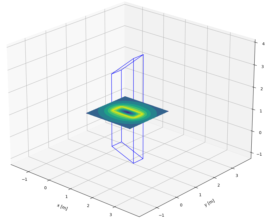
The tapering at either end of the current source is to facilitate treatment of curvilinear circuits. As the tapering is only in one plane however, this treatment is only directly applicable to planar curvilinear circuits.
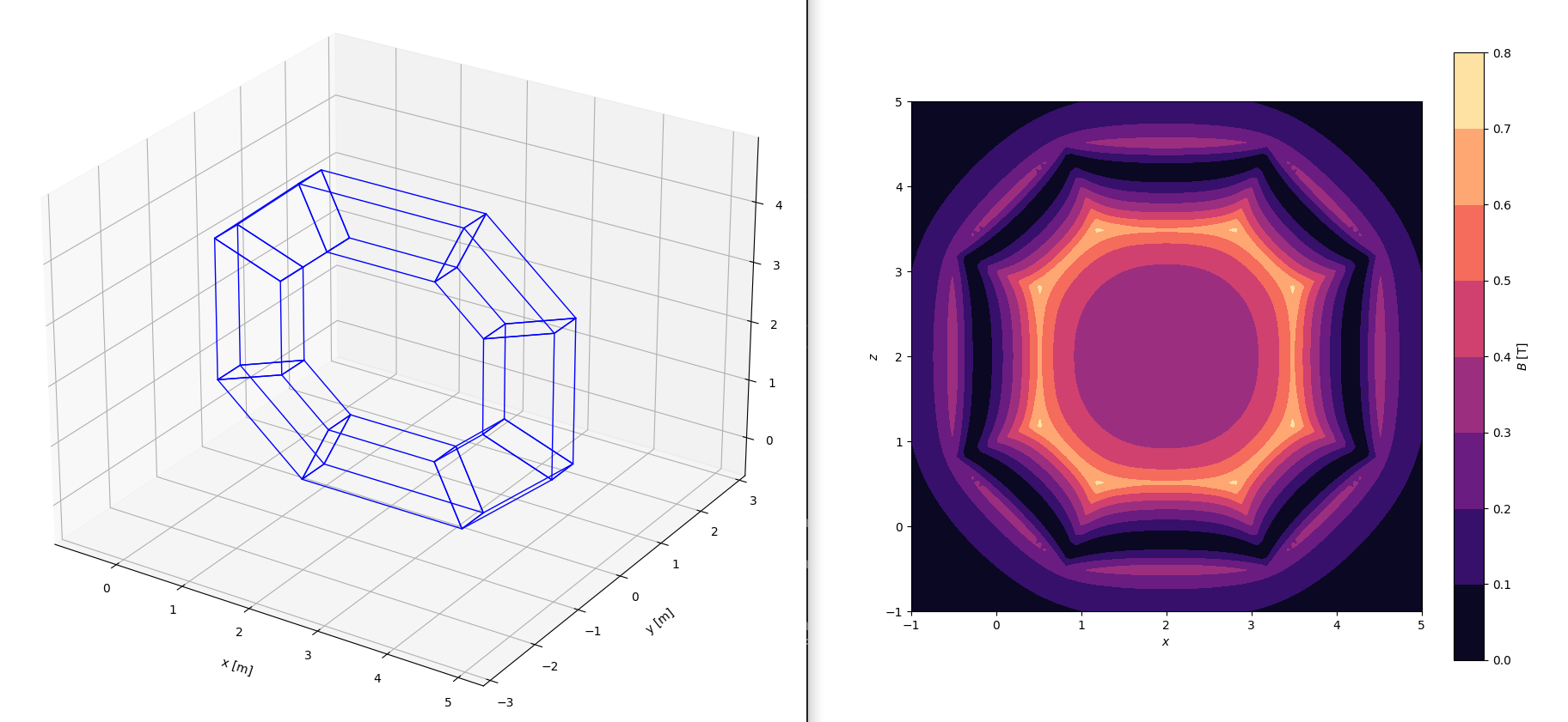
The ArbitraryPlanarRectangularXSCircuit is a utility provided to enable the user to
easily set up a planar circuit with a rectangular cross-section using
TrapezoidalPrismCurrentSource objects.
import matplotlib.pyplot as plt
import numpy as np

from bluemira.magnetostatics.circuits import ArbitraryPlanarRectangularXSCircuit

x = np.array([0, 1, 3, 4, 4, 3, 1, 0, 0])
y = np.zeros(len(x))
z = np.array([1, 0, 0, 1, 3, 4, 4, 3, 1])

source = ArbitraryPlanarRectangularXSCircuit(
    shape=np.c_[x, y, z], breadth=0.5, depth=0.25, current=1e6
)

x = np.linspace(-1, 5, 100)
z = np.linspace(-1, 5, 100)
xx, zz = np.meshgrid(x, z)

Bx, By, Bz = source.field(xx, np.zeros_like(xx), zz)
B = np.sqrt(Bx**2 + By**2 + Bz**2)
source.plot()
f, ax = plt.subplots()
cm = ax.contourf(xx, zz, B, cmap="magma")
f.colorbar(cm, label="$B$ [T]")
ax.set_aspect("equal")
ax.set_xlabel("$x$")
ax.set_ylabel("$z$")
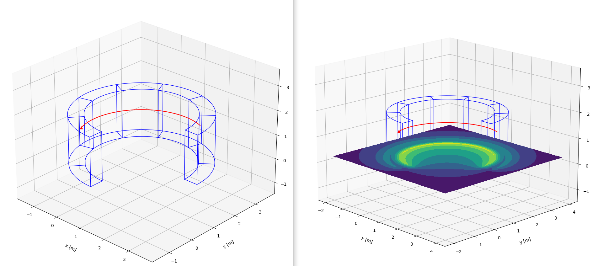
Circular arcs
A CircularArcCurrentSource object is used for circular arcs of uniform current
density. The magnetic field can be calculated at any point, following equations
described in [Feng_1985].
import matplotlib.pyplot as plt
import numpy as np

from bluemira.magnetostatics.circular_arc import CircularArcCurrentSource

source = CircularArcCurrentSource(
    origin=[1, 1, 1],
    ds=[1, 0, 0],
    normal=[0, 1, 0],
    t_vec=[0, 0, 1],
    breadth=0.25,
    depth=1,
    radius=2,
    dtheta=270,
    current=1e6,
)

x = np.linspace(-2, 4, 100)
y = np.linspace(-2, 4, 100)
xx, yy = np.meshgrid(x, y)


# Calculate field values in global x, y, z Cartesian coordinates.
Bx, By, Bz = source.field(xx, yy, 0.25 * np.ones_like(xx))
B = np.sqrt(Bx**2 + By**2 + Bz**2)

source.plot()
ax = plt.gca()
ax.contourf(xx, yy, B, zdir="z", offset=0.25)
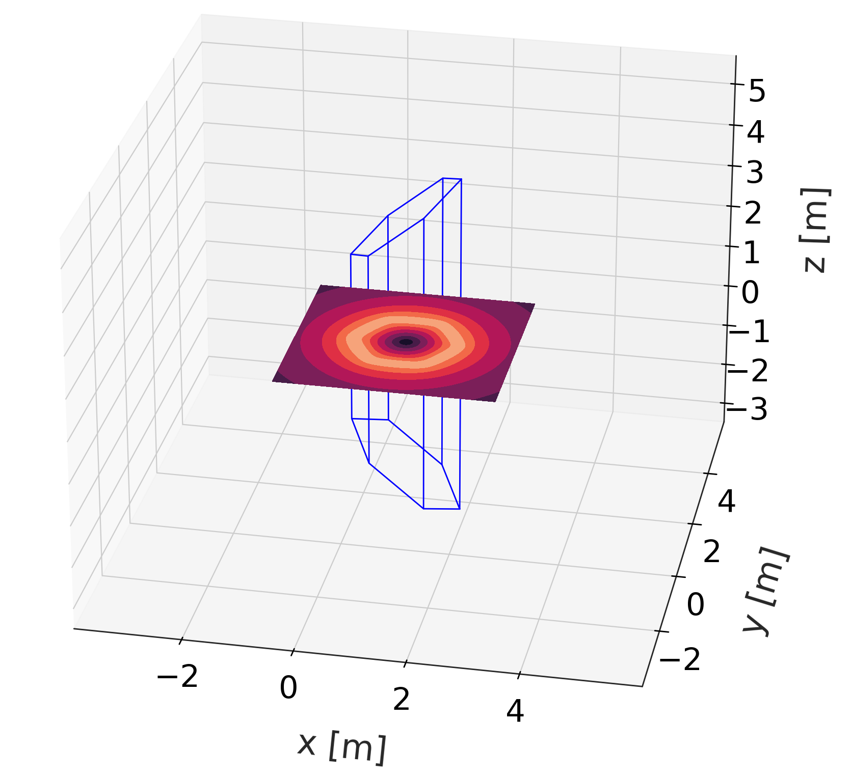
Volume integral method
The magnetic field due to a uniform current density distribution \(\mathbf{J}\) in a volume \(V\) can be written as:
Following a procedure described in [Fabbri_2008], this volume integral can be solved by a series of surface integrals, which themselves can be solved as a series of line integrals.
A PolyhedralPrismCurrentSource object is used to describe a conductor segment of
uniform current density, with an arbitary (polygonal) cross-section.
import matplotlib.pyplot as plt
import numpy as np

from bluemira.geometry.coordinates import Coordinates
from bluemira.magnetostatics.polyhedral_prism import PolyhedralPrismCurrentSource

s = 0.5
d = 0.5 * np.sqrt(3)
x = np.array([2 * s, s, -s, -2 * s, -s, s])
y = np.zeros(6)
z = np.array([0, d, d, 0, -d, -d])

source = PolyhedralPrismCurrentSource(
    origin=[1, 1, 1],  # the centroid of the current source
    ds=[0, 0, 6],  # length of the source is determined by the norm of ds
    normal=[0, 1, 0],
    t_vec=[1, 0, 0],
    xs_coordinates=Coordinates(np.c_[x, y, z]),  # Points specified in x-z
    alpha=45.0,  # angle at the tip of the current source
    beta=45,  # angle at the tail of the current source (must be the same!)
    current=1e6,
)

x = np.linspace(0, 4, 100) - 1
y = np.linspace(0, 4, 100) - 1
xx, yy = np.meshgrid(x, y)

# Calculate field values in global x, y, z Cartesian coordinates.
Bx, By, Bz = source.field(xx, yy, np.ones_like(xx))
B = np.sqrt(Bx**2 + By**2 + Bz**2)

source.plot()
ax = plt.gca()
ax.contourf(xx, yy, B, zdir="z", offset=1)
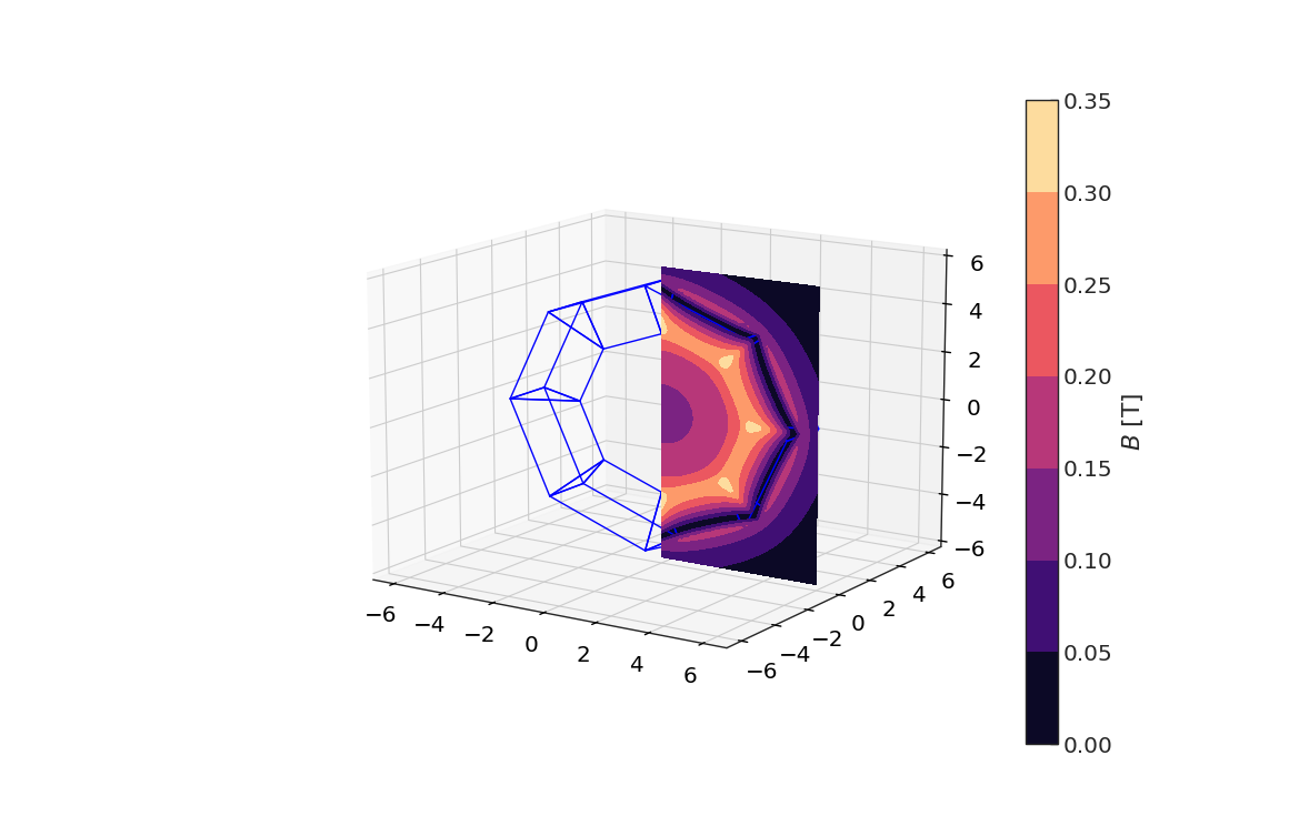
Tapering at the ends of the current source allows for the facilitation of circuits,
like with the trapezoidal current source. The
ArbitraryPlanarPolyhedralXSCircuit is a utility provided to enable the construction
of planar circuits, making use of the PolyhedralPrismCurrentSource object.
Note
Sadly, the PolyhedralPrismCurrentSource can only handle equal angle end-caps.
This is due to a limitation of the formulation that will hopefully be resolved in
future.
import matplotlib.pyplot as plt
import numpy as np

from bluemira.geometry.coordinates import Coordinates
from bluemira.geometry.tools import make_circle
from bluemira.magnetostatics.circuits import ArbitraryPlanarPolyhedralXSCircuit

ring = make_circle(
    radius=4, center=[0, 0, 0], start_angle=0, end_angle=360, axis=[0, 1, 0]
)
xs = Coordinates({"x": [-1, 1, 1, -1], "z": [0, 1, -1, 0]})
xs.translate(xs.center_of_mass)
source = ArbitraryPlanarPolyhedralXSCircuit(ring.discretise(ndiscr=9), xs, current=1e6)

x = np.linspace(0, 6, 100)
z = np.linspace(-6, 6, 100)
xx, zz = np.meshgrid(x, z)

Bx, By, Bz = source.field(xx, np.zeros_like(xx), zz)
B = np.sqrt(Bx**2 + By**2 + Bz**2)
f = plt.figure()
ax = f.add_subplot(1, 1, 1, projection="3d")
source.plot(ax)
cm = ax.contourf(xx, B, zz, cmap="magma", zdir="y", offset=0)
f.colorbar(cm, label="$B$ [T]")
Finite element
The implementation of the magnetostatic Finite Element solver is limited to 2D axially symmetric problems. In such an approximation, the Maxwell equations, as function of the poloidal magnetic flux (\(\Psi\)), are reduced to the form ([Zohm_2015], page 25):
whose weak formulation, considering null Dirichlet boundary conditions, is defined as ([Villone_2013]):
where \(v\) is the basis element function of the defined functional subspace \(V\).
import time
from pathlib import Path
import gmsh
import matplotlib.pyplot as plt
import numpy as np
from dolfinx.io import XDMFFile
from matplotlib.axes import Axes
from mpi4py import MPI
from bluemira.base.components import Component, PhysicalComponent
from bluemira.base.file import get_bluemira_path
from bluemira.geometry.face import BluemiraFace
from bluemira.geometry.tools import make_polygon
from bluemira.geometry.wire import BluemiraWire
from bluemira.magnetostatics import greens
from bluemira.magnetostatics.biot_savart import Bz_coil_axis
from bluemira.magnetostatics.fem_utils import (
Association,
create_j_function,
model_to_mesh,
)
from bluemira.magnetostatics.finite_element_2d import FemMagnetostatic2d
from bluemira.mesh import meshing
ri = 0.01 # Inner radius of copper wire
rc = 5 # Outer radius of copper wire
R = 25 # Radius of domain
R_ext = 250
I_wire = 1e6 # wire's current
gdim = 2 # Geometric dimension of the mesh
# Define geometry for wire cylinder
nwire = 20 # number of wire divisions
lwire = 0.1 # mesh characteristic length for each segment
nenclo = 20 # number of external enclosure divisions
lenclo = 0.5 # mesh characteristic length for each segment
lcar_axis = 0.1 # axis characteristic length
# enclosure
theta_encl = np.linspace(np.pi / 2, -np.pi / 2, nenclo)
r_encl = R * np.cos(theta_encl)
z_encl = R * np.sin(theta_encl)
# adding (0,0) to improve mesh quality
enclosure_points = np.array([
[0, 0, 0],
*[[r_encl[ii], z_encl[ii], 0] for ii in range(r_encl.size)],
])
nenclo_ext = 40
lenclo_ext = 20
# external enclosure
theta_encl_ext = np.linspace(np.pi / 2, -np.pi / 2, nenclo_ext)
r_encl_ext = R_ext * np.cos(theta_encl_ext)
z_encl_ext = R_ext * np.sin(theta_encl_ext)
enclosure_points_ext1 = np.array([
*[[r_encl_ext[ii], z_encl_ext[ii], 0] for ii in range(r_encl_ext.size)]
])
enclosure_points_ext2 = enclosure_points[1:][::-1]
poly_enclo_ext = make_polygon(
np.concatenate((enclosure_points_ext1, enclosure_points_ext2)), closed=True
)
poly_enclo_ext.mesh_options = {"lcar": lenclo_ext, "physical_group": "poly_enclo_ext"}
enclosure_ext = BluemiraFace([poly_enclo_ext])
enclosure_ext.mesh_options.physical_group = "enclo_ext"
poly_enclo1 = make_polygon(enclosure_points[0:2])
poly_enclo1.mesh_options = {"lcar": lcar_axis, "physical_group": "poly_enclo1"}
poly_enclo2 = make_polygon(enclosure_points[1:])
poly_enclo2.mesh_options = {"lcar": lenclo, "physical_group": "poly_enclo2"}
poly_enclo3 = make_polygon(np.array([enclosure_points[-1], enclosure_points[0]]))
poly_enclo3.mesh_options = {"lcar": lcar_axis, "physical_group": "poly_enclo3"}
poly_enclo = BluemiraWire([poly_enclo1, poly_enclo2, poly_enclo3])
poly_enclo.close("poly_enclo")
poly_enclo.mesh_options = {"lcar": lenclo, "physical_group": "poly_enclo"}
# coil
theta_coil = np.linspace(0, 2 * np.pi, nwire)
r_coil = rc + ri * np.cos(theta_coil[:-1])
z_coil = ri * np.sin(theta_coil)
coil_points = [[r_coil[ii], z_coil[ii], 0] for ii in range(r_coil.size)]
poly_coil = make_polygon(coil_points, closed=True)
lcar_coil = np.ones([poly_coil.vertexes.shape[1], 1]) * lwire
poly_coil.mesh_options = {"lcar": lwire, "physical_group": "poly_coil"}
coil = BluemiraFace([poly_coil])
coil.mesh_options.physical_group = "coil"
enclosure = BluemiraFace([poly_enclo, poly_coil])
enclosure.mesh_options.physical_group = "enclo"
c_universe = Component(name="universe")
c_enclo_ext = PhysicalComponent(
name="enclosure_Ext", shape=enclosure_ext, parent=c_universe
)
c_enclo = PhysicalComponent(name="enclosure", shape=enclosure, parent=c_universe)
c_coil = PhysicalComponent(name="coil", shape=coil, parent=c_universe)
directory = get_bluemira_path("", subfolder="generated_data")
meshfiles = [Path(directory, p).as_posix() for p in ["Mesh.geo_unrolled", "Mesh.msh"]]
meshing.Mesh(meshfile=meshfiles)(c_universe, dim=2)
(mesh, ct, ft), labels = model_to_mesh(gmsh.model, gdim=2)
gmsh.write("Mesh.msh")
gmsh.finalize()
with XDMFFile(MPI.COMM_WORLD, "mt.xdmf", "w") as xdmf:
xdmf.write_mesh(mesh)
xdmf.write_meshtags(ft, mesh.geometry)
xdmf.write_meshtags(ct, mesh.geometry)
em_solver = FemMagnetostatic2d(2)
em_solver.set_mesh(mesh, ct)
coil_tag = labels["coil"][1]
functions = [(1, coil_tag, I_wire)]
jtot = create_j_function(mesh, ct, [Association(1, coil_tag, I_wire)])
em_solver.define_g(jtot)
em_solver.solve()
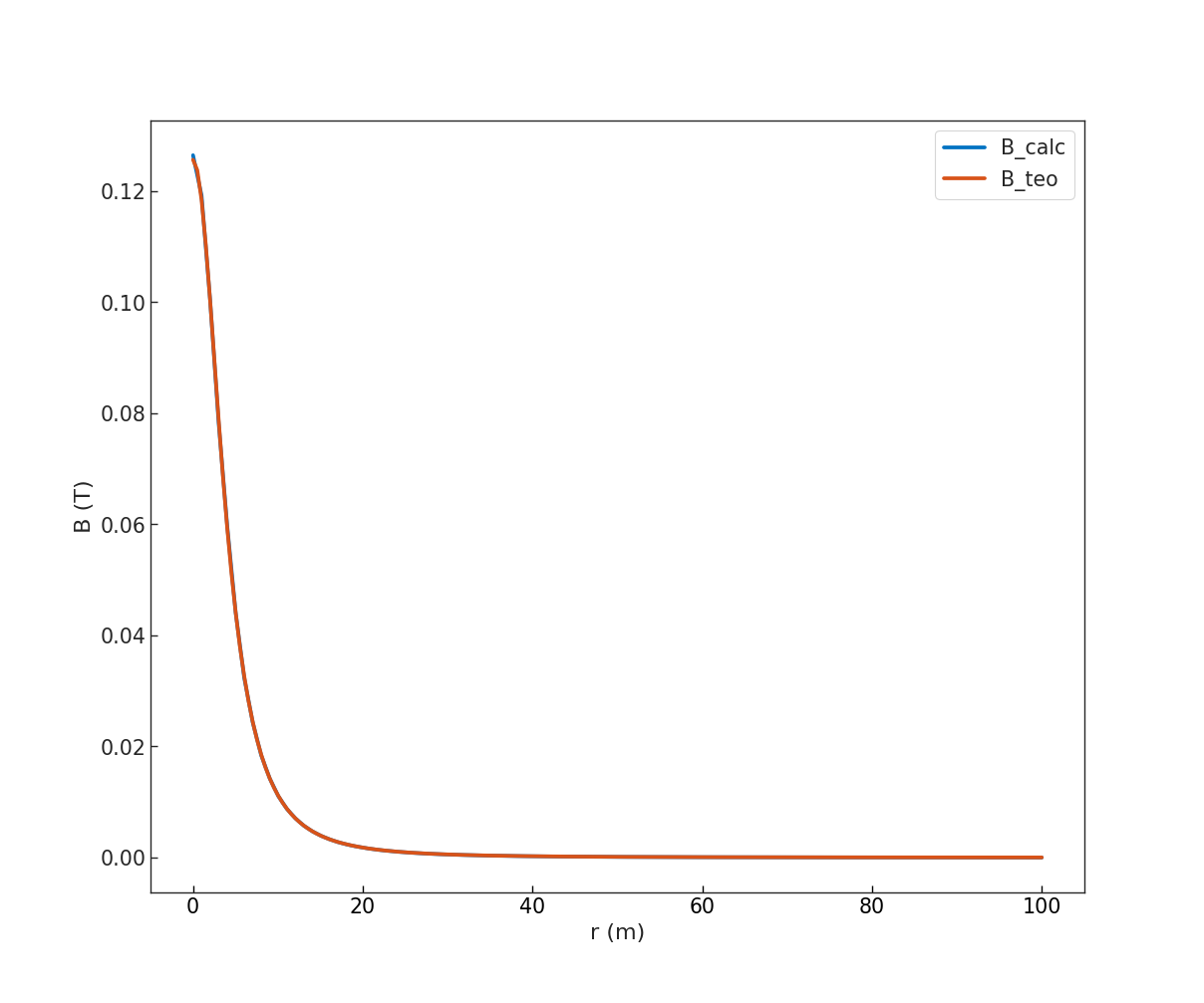
# Compare the obtained B with both the theoretical value
#
# 1) Along the z axis (analytical solution)
r_offset = 2 * lcar_axis
z_points_axis = np.linspace(0, R, 200)
r_points_axis = np.zeros(z_points_axis.shape) + r_offset
b_points = np.array([r_points_axis, z_points_axis, 0 * z_points_axis]).T
Bz_axis = em_solver.calculate_b()(b_points)
Bz_axis = Bz_axis[:, 1]
bz_points = b_points[:, 1]
B_z_teo = np.array([Bz_coil_axis(rc, 0, z, I_wire) for z in bz_points])
ax: Axes
_, ax = plt.subplots()
ax.plot(bz_points, Bz_axis, label="B_calc")
ax.plot(bz_points, B_z_teo, label="B_teo")
ax.set_xlabel("r (m)")
ax.set_ylabel("B (T)")
ax.legend()
plt.show()
_, ax = plt.subplots()
ax.plot(bz_points, Bz_axis - B_z_teo, label="B_calc - B_teo")
ax.set_xlabel("r (m)")
ax.set_ylabel("error (T)")
ax.legend()
plt.show()
# 2) Along a radial path at z_offset (solution from green function)
z_offset = 100 * ri
points_x = np.linspace(r_offset, R, 200)
points_z = np.zeros(z_points_axis.shape) + z_offset
new_points = np.array([points_x, points_z, 0 * points_z]).T
new_points = new_points[1:]
B_fem = em_solver.calculate_b()(new_points)
Bx_fem = B_fem.T[0]
Bz_fem = B_fem.T[1]
g_psi, g_bx, g_bz = greens.greens_all(rc, 0, new_points[:, 0], new_points[:, 1])
g_psi *= I_wire
g_bx *= I_wire
g_bz *= I_wire
_, ax = plt.subplots()
ax.plot(new_points[:, 0], Bx_fem, label="Bx_fem")
ax.plot(new_points[:, 0], g_bx, label="Green Bx")
ax.set_xlabel("r (m)")
ax.set_ylabel("Bx (T)")
ax.legend()
plt.show()
_, ax = plt.subplots()
ax.plot(new_points[:, 0], Bz_fem, label="Bz_fem")
ax.plot(new_points[:, 0], g_bz, label="Green Bz")
ax.set_xlabel("r (m)")
ax.set_ylabel("Bz (T)")
ax.legend()
plt.show()
_, ax = plt.subplots()
ax.plot(new_points[:, 0], Bx_fem - g_bx, label="Bx_calc - GreenBx")
ax.plot(new_points[:, 0], Bz_fem - g_bz, label="Bz_calc - GreenBz")
ax.legend()
ax.set_xlabel("r (m)")
ax.set_ylabel("error (T)")
plt.show()
References
Zhang, C. S. Koh, An Efficient Semianalytic Computation Method of Magnetic Field for a Circular Coil With Rectangular Cross Section, IEEE Transactions on Magnetics, 2012, pp. 62-68 DOI: 10.1109/TMAG.2011.2167981
Babic and C. Aykel, An improvement in the calculation of the magnetic field for an arbitrary geometry coil with rectangular cross section, International Journal of Numerical Modelling, Electronic Networks, Devices and Fields, 2005, vol. 18, pp. 493-504 DOI: 10.1002/jnm.594
Babic and C. Aykel, An improvement in the calculation of the magnetic field for an arbitrary geometry coil with rectangular cross section - Erratum, International Journal of Numerical Modelling, Electronic Networks, Devices and Fields, 2005
Feng, The treatment of singularities in calculation of magnetic field using integral method, IEEE Transactions on Magnetics, 1985, vol. 21 DOI: 10.1109/TMAG.1985.1064259
Fabbri, Magnetic Flux Density and Vector Potential of Uniform Polyhedral Sources, IEEE Transactions on Magnetics, 2008, vol. 44, no. 1 DOI: 10.1109/TMAG.2007.908698
Zohm, Magnetohydrodynamic Stability of Tokamaks, Wiley-VCH, Germany, 2015 DOI: 10.1002/9783527677375
VILLONE, F. et al. Plasma Phys. Control. Fusion 55 (2013) 095008, DOI: 10.1088/0741-3335/55/9/095008