utilities

Toroidal coordinate transform

This is a demonstration of the conversion between cylindrical and toroidal coordinate systems using the bluemira functions cylindrical_to_toroidal and toroidal_to_cylindrical. We denote toroidal coordinates by (\(\tau\), \(\sigma\), \(\phi\)) and cylindrical coordinates by (\(R\), \(z\), \(\phi\)).

The snippets in this document use these imports

import matplotlib.pyplot as plt
import numpy as np

from bluemira.utilities.tools import (
    cylindrical_to_toroidal,
    toroidal_to_cylindrical,
)

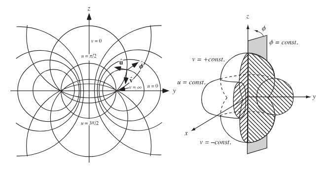
This diagram is taken from Wolfram MathWorld and shows a toroidal coordinate system. It uses (\(u\), \(v\), \(\phi\)) whereas we use (\(\tau\), \(\sigma\), \(\phi\)).

In toroidal coordinates, surfaces of constant \(\tau\) are non-intersecting tori of different radii, and surfaces of constant \(\sigma\) are non-concentric spheres of different radii which intersect the focal ring.

We are working in the poloidal plane, so we set \(\phi = 0\), and so are looking at a bipolar coordinate system. We are transforming about a focus \((R_0, Z_0)\) in the poloidal plane.

Here, curves of constant \(\tau\) are non-intersecting circles of different radii that surround the focus and curves of constant \(\sigma\) are non-concentric circles which intersect at the focus.

To transform from toroidal coordinates to cylindrical coordinates about the focus in the poloidal plant \((R_0, Z_0)\), we have the following relations:

\[\begin{split}R = R_0 \frac{\sinh\tau}{\cosh\tau - \cos\sigma}\\ z - Z_0 = R_0 \frac{\sin\tau}{\cosh\tau - \cos\sigma}\end{split}\]

where we have \(0 \le \tau < \infty\) and \(-\pi < \sigma \le \pi\).

The inverse transformations are given by:

\[\tau = \ln \frac{d_1}{d_2}\]

\[\sigma = \text{sign}(z - Z_0) \arccos \frac{d_1^2 + d_2^2 - 4 R_0^2}{2 d_1 d_2}\]

where we have

\[\begin{split}d_1^2 = (R + R_0)^2 + (z - Z_0)^2\\ d_2^2 = (R - R_0)^2 + (z - Z_0)^2\end{split}\]

Converting a unit circle

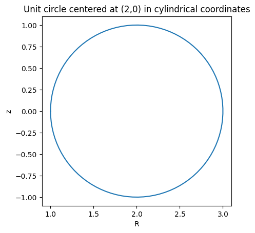
We will start with an example of converting a unit circle in cylindrical coordinates to toroidal coordinates and then converting back to cylindrical using the bluemira functions cylindrical_to_toroidal and toroidal_to_cylindrical. This unit circle is centered at the point (2,0) in the poloidal plane.

Original circle:

theta = np.linspace(-np.pi, np.pi, 100)
x = 2 + np.cos(theta)
y = np.sin(theta)
plt.plot(x, y)
plt.title("Unit circle centered at (2,0) in cylindrical coordinates")
plt.xlabel("R")
plt.ylabel("z")
plt.axis("square")
plt.show()

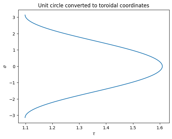
Convert this circle to toroidal coordinates:

tau, sigma = cylindrical_to_toroidal(R=x, R_0=2, Z=y, Z_0=0)
plt.plot(tau, sigma)
plt.title("Unit circle converted to toroidal coordinates")
plt.xlabel(r"$\tau$")
plt.ylabel(r"$\sigma$")
plt.show()

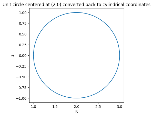
Convert this back to cylindrical coordinates to recover the original unit circle centered at (2,0) in the poloidal plane:

rs, zs = toroidal_to_cylindrical(R_0=2, Z_0=0, tau=tau, sigma=sigma)
plt.plot(rs, zs)
plt.title("Unit circle centered at (2,0) converted back to cylindrical coordinates")
plt.xlabel("R")
plt.ylabel("z")
plt.axis("square")

Curves of constant \(\tau\) and \(\sigma\)

When plotting in cylindrical coordinates, curves of constant \(\tau\) correspond to non-intersecting circles that surround the focus \((R_0, Z_0)\), and curves of constant \(\sigma\) correspond to non-concentric circles that intersect at the focus.

Curves of constant \(\tau\) plotted in both cylindrical and toroidal coordinates

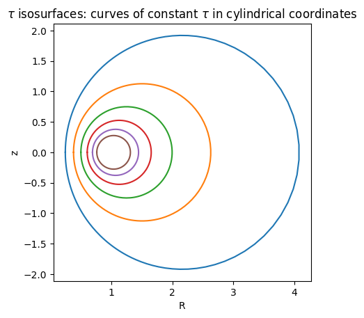
Set the focus point to be \((R_0, Z_0) = (1,0)\). We plot 6 curves of constant \(\tau\) in cylindrical coordinates

# Define the focus point
R_0 = 1
Z_0 = 0

# Create array of 6 tau values, 6 curves of constant tau will be plotted
tau = np.linspace(0.5, 2, 6)
sigma = np.linspace(-np.pi, np.pi, 200)

rlist = []
zlist = []
# Plot the curve in cylindrical coordinates for each constant value of tau
for t in tau:
    rs, zs = toroidal_to_cylindrical(R_0=R_0, Z_0=Z_0, sigma=sigma, tau=t)
    rlist.append(rs)
    zlist.append(zs)
    plt.plot(rs, zs)

plt.axis("square")
plt.xlabel("R")
plt.ylabel("z")
plt.title(r"$\tau$ isosurfaces: curves of constant $\tau$ in cylindrical coordinates")
plt.show()

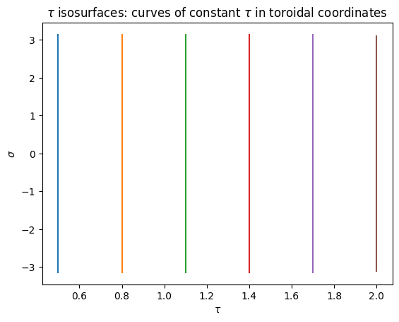
Now convert to toroidal coordinates using cylindrical_to_toroidal and plot - here curves of constant \(\tau\) are straight lines

taulist = []
sigmalist = []
for i in range(len(rlist)):
    tau, sigma = cylindrical_to_toroidal(R_0=R_0, Z_0=Z_0, R=rlist[i], Z=zlist[i])
    taulist.append(tau)
    sigmalist.append(sigma)
    plt.plot(tau, sigma)

plt.xlabel(r"$\tau$")
plt.ylabel(r"$\sigma$")
plt.title(r"$\tau$ isosurfaces: curves of constant $\tau$ in toroidal coordinates")
plt.show()

Curves of constant \(\sigma\) plotted in both cylindrical and toroidal coordinates

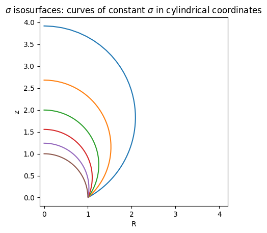
Set the focus point to be \((R_0, Z_0) = (1,0)\). We plot 6 curves of constant \(\sigma\) in cylindrical coordinates

# Define the focus point
R_0 = 1
Z_0 = 0

# Create array of 6 sigma values, 6 curves of constant sigma will be plotted
sigma = np.linspace(0.5, np.pi / 2, 6)
tau = np.linspace(0, 5, 200)

rlist = []
zlist = []
# Plot the curve in cylindrical coordinates for each constant value of sigma
for s in sigma:
    rs, zs = toroidal_to_cylindrical(R_0=R_0, Z_0=Z_0, sigma=s, tau=tau)
    rlist.append(rs)
    zlist.append(zs)
    plt.plot(rs, zs)

plt.axis("square")
plt.xlabel("R")
plt.ylabel("z")
plt.title(
    r"$\sigma$ isosurfaces: curves of constant $\sigma$ in cylindrical coordinates"
)
plt.show()

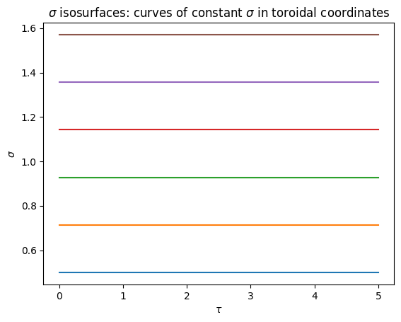
Now convert to toroidal coordinates using cylindrical_to_toroidal and plot - here curves of constant \(\sigma\) are straight lines

taulist = []
sigmalist = []
for i in range(len(rlist)):
    tau, sigma = cylindrical_to_toroidal(R_0=R_0, Z_0=Z_0, R=rlist[i], Z=zlist[i])
    taulist.append(tau)
    sigmalist.append(sigma)
    plt.plot(tau, sigma)

plt.xlabel(r"$\tau$")
plt.ylabel(r"$\sigma$")
plt.title(r"$\sigma$ isosurfaces: curves of constant $\sigma$ in toroidal coordinates")
plt.show()